Note
Go to the end to download the full example code.
Fourier Local Correlation Tracking#
This example applies Fourier Local Correlation Tracking (FLCT)
to a set of two arrays using pyflct.
import matplotlib.pyplot as plt
import numpy as np

import pyflct
This examples demonstrates how to find the 2D velocity flow field.
It has three parts all of which depicts motion of the object in a dummy
image in some particular directions.
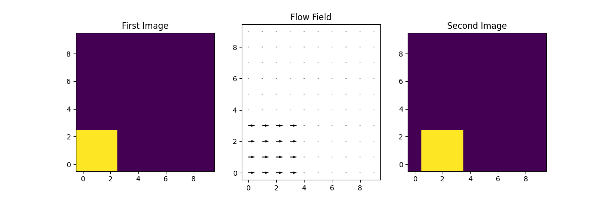
First we plot the velocity field when the image moves in positive X direction.
Now we will apply the FLCT.
The values of the parameters used gave the best visual result
of the velocities. The time difference between the two images, deltat is
1 second. The units of length of the side of a single pixel, deltas is
1. The width of Gaussian used to weigh the subimages, sigma is taken to be 2.3.
Note you should experiment with the values of sigma to get the best results.
We will plot the 2D flow field what we get when the image have moved in positive X direction.
# But first we need to create a meshgrid on which the flow field will be plotted
X = np.arange(0, 10, 1)
Y = np.arange(0, 10, 1)
U, V = np.meshgrid(X, Y)

# Plotting the first image
fig = plt.figure(figsize=(12, 4))

ax1 = fig.add_subplot(131)
plt.imshow(image1, origin="lower")
ax1.set_title("First Image")

# Plot the 2D flow field
ax2 = fig.add_subplot(132)
ax2.quiver(U, V, vel_x, vel_y, scale=20)
ax2.set_title("Flow Field")

# Plot the shifted image
ax3 = fig.add_subplot(133)
plt.imshow(image2, origin="lower")
ax3.set_title("Second Image")
Text(0.5, 1.0, 'Second Image')
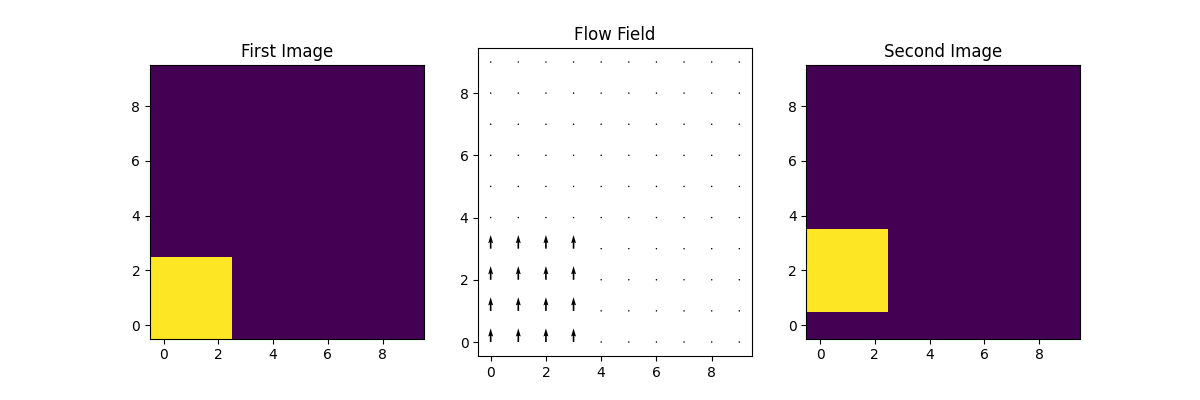
Now, we plot the velocity field when the image moves in positive Y direction.
Now we again apply FLCT to this new set of images using the same parameter values as before.
We will plot the 2D flow field what we get when the image have moved in positive Y direction.
# Plotting the first image
fig = plt.figure(figsize=(12, 4))

ax1 = fig.add_subplot(131)
plt.imshow(image1, origin="lower")
ax1.set_title("First Image")

# Plot the 2D flow field
ax2 = fig.add_subplot(132)
ax2.quiver(U, V, vel_x, vel_y, scale=20)
ax2.set_title("Flow Field")

# Plot the shifted image
ax3 = fig.add_subplot(133)
plt.imshow(image2, origin="lower")
ax3.set_title("Second Image")
Text(0.5, 1.0, 'Second Image')
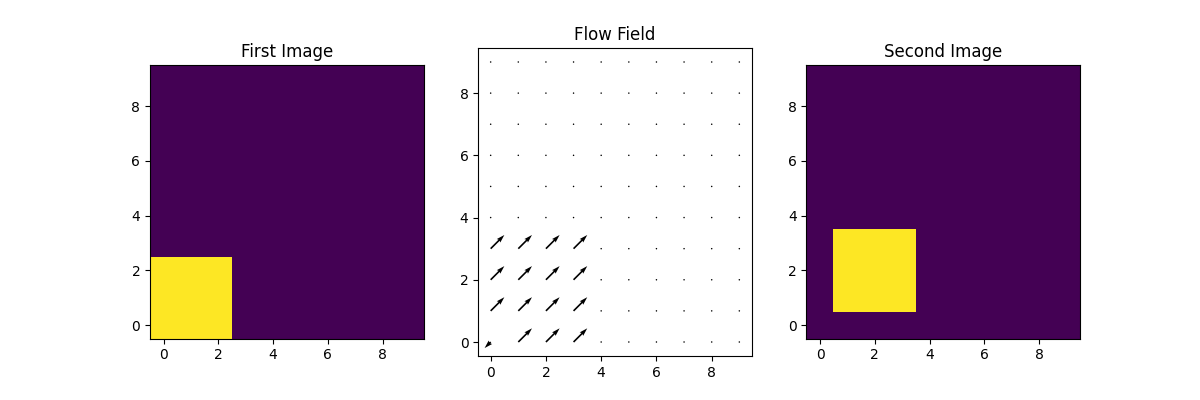
Finally we plot the velocity field when the image moves in both the directions.
We again apply FLCT with the similar settings as before to find the velocity field
We will plot the 2D flow field what we get when the image have moved in both directions.
# Plotting the first image
fig = plt.figure(figsize=(12, 4))

ax1 = fig.add_subplot(131)
plt.imshow(image1, origin="lower")
ax1.set_title("First Image")

# Plot the 2D flow field
ax2 = fig.add_subplot(132)
ax2.quiver(U, V, vel_x, vel_y, scale=20)
ax2.set_title("Flow Field")

# Plot the shifted image
ax3 = fig.add_subplot(133)
plt.imshow(image2, origin="lower")
ax3.set_title("Second Image")
Text(0.5, 1.0, 'Second Image')
Notice the lonely pixel in the bottom left of every flow field which has value less than zero.
This discrepancy is due one of the limitations of the FLCT algorithm where it is unable to reliably
calculate the velocities within sigma pixels of the image edges.
plt.show()
Total running time of the script: (0 minutes 0.339 seconds)